TRIM Google Sheets Function [With Quiz]
 Updated: October 18, 2021
 In Google Sheets the TRIM function removes leading, trailing, and repeated spaces from text.
In other words, it removes all spaces from the text, leaving a single space between words.
TRIM Syntax
- text = the "text" or a cell reference to the text you want to remove the leading, trailing, and repeated spaces from.
This function is useful for cleaning up user-submitted text to a consistent format.
For some reason people often add unnecessary spaces when entering text into fields. If you don't account for this, other functions and formulas in your sheet can throw errors.


FREE RESOURCE
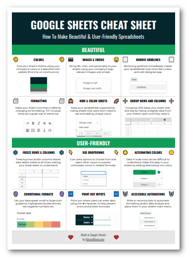
Google Sheets Cheat Sheet
12 exclusive tips to make user-friendly sheets from today:

You'll get updates from me with an easy-to-find "unsubscribe" link.
TRIM Function Example
| A | B | C | |
| 1 | Text | Formula | Output |
| 2 | Pete Miller | =TRIM(A2) | Pete Miller |
| 3 | 100 Example St | =TRIM(A3) | 100 Example Street |
| 4 | Scranton, PA | =TRIM(A4) | PA |
You can also reference text directly instead of using a cell reference:
Will output: 100 Example Street
Using The TRIM Function On A Whole Column
By combining the TRIM function and the ArrayFormula function you can force TRIM to accept more than one argument.
This means you can clean multiple cells of text, an entire column or row, or even a table with only one formula.
Here's an example using the same data as above:
| A | B | C | |
| 1 | Text | Formula | Output |
| 2 | Pete Miller | =ArrayFormula(TRIM(A2:A4)) | Pete Miller |
| 3 | 100 Example St | 100 Example Street | |
| 4 | PA | PA |
All of the text has the unnecessary spaces removed using a single formula.
TRIM Errors
TRIM is a stable function, handling the following without error:
- Blank cells,
- Numbers (returning them as text), and
- Boolean data (returning them as text)
For images in cells and sparklines, TRIM returns a blank cell.
If you input a range (e.g. A2:A4) without using ArrayFormula it will output one piece of cleaned text if the range crosses the same row or column as the formula's cell.
Otherwise, it will throw a #VALUE! error:
An array value could not be found.
TRIM requires exactly one argument (a value, cell reference, or range reference).
If you have no arguments or more than one you will receive a #N/A error:
Wrong number of arguments to TRIM. Expected 1 arguments, but got 2 arguments.
TRIM Function Quiz
Here's a quick summary of how to use the quiz spreadsheet:
- Select the required cell while the formula bar is empty
- Type your answer in the formula bar
- You can click on the spreadsheet to add cell/range references
Complete all questions to solidify your understanding of the TRIM function.
| A | B | C | |
| 1 | Original | Trimmed Cell | Trimmed Column |
| 2 | Jim Halpert | ||
| 3 | 363 Linden Ave | ||
| 4 | Scranton, PA | ||
| 5 | |||
| 6 | |||
| 7 |


FREE RESOURCE
Google Sheets Cheat Sheet
12 exclusive tips to make user-friendly sheets from today:

You'll get updates from me with an easy-to-find "unsubscribe" link.

![MAX Google Sheets Function [With Quiz]](https://kierandixon.com/wp-content/uploads/max-function-google-sheets.png)

![SUMIF Google Sheets Function [With Quiz]](https://kierandixon.com/wp-content/uploads/sumif-google-sheets-function.png)