How To Highlight Duplicates In Google Sheets
 Updated: August 31, 2021
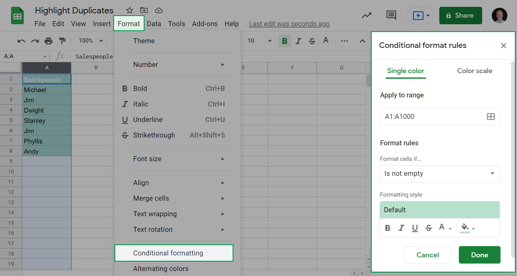
 - Highlight the columns in which you want to highlight duplicates
- Go to ➜ in the main menu to bring up the Conditional format rules sidebar
- In the Format cells if… dropdown select and enter one of the formulas below
- Choose your desired Formatting style and click Done
Custom formula to highlight duplicate values in single cells:
Custom formula to highlight duplicate rows:
You'll need to adjust the cell and range references to match your highlighted columns.
Keep reading for a detailed description about how each of these formulas works.
You can highlight duplicate entries in Google Sheets using conditional formatting to change the color of the cell.
Which do you need to do? Highlighting duplicates based on:
- A single cell's value
- Including the first instance (read this to learn the most)
- Excluding the first instance
- A whole row's contents
Highlighting Duplicates In One Column In Google Sheets
Duplicates are values that appear more than once.
This makes finding and highlighting them using conditional formatting relatively easy… with the right formula.
Conditional formatting is a BIG topic. I'm only going to touch on the relevant parts here.
Here's an example of a column with a duplicate entry:
| A | |
| 1 | Salespeople |
| 2 | Michael |
| 3 | Jim |
| 4 | Dwight |
| 5 | Stanley |
| 6 | Jim |
| 7 | Phyllis |
| 8 | Andy |
What's a formula that counts if each entry occurs more than once?
How about the appropriately named:
- range = the range reference or array that is tested against the criterion
- criterion = a logic test or matching pattern applied to the range
You can input the range of names from the example above and provide each individual name as a criterion:
| A | B | C | |
| 1 | Salespeople | Formula | Output |
| 2 | Michael | =COUNTIF(A2:A8, A2) | 1 |
| 3 | Jim | =COUNTIF(A2:A8, A3) | 2 |
| 4 | Dwight | =COUNTIF(A2:A8, A4) | 1 |
| 5 | Stanley | =COUNTIF(A2:A8, A5) | 1 |
| 6 | Jim | =COUNTIF(A2:A8, A6) | 2 |
| 7 | Phyllis | =COUNTIF(A2:A8, A7) | 1 |
| 8 | Andy | =COUNTIF(A2:A8, A8) | 1 |
Now you know which entries are duplicates, but this won't highlight them.
Why?
When designing a formula for conditional formatting you need the output to be TRUE or FALSE.
Work a logic test into your conditional formatting formulas to make sure of this.
You need to write a formula that uses a logic test to output either TRUE or FALSE.
What if you alter the current formula to test if its output is greater than 1:
| A | B | C | |
| 1 | Salespeople | Formula | Output |
| 2 | Michael | =COUNTIF(A2:A8, A2)>1 | FALSE |
| 3 | Jim | =COUNTIF(A2:A8, A3)>1 | TRUE |
| 4 | Dwight | =COUNTIF(A2:A8, A4)>1 | FALSE |
| 5 | Stanley | =COUNTIF(A2:A8, A5)>1 | FALSE |
| 6 | Jim | =COUNTIF(A2:A8, A6)>1 | TRUE |
| 7 | Phyllis | =COUNTIF(A2:A8, A7)>1 | FALSE |
| 8 | Andy | =COUNTIF(A2:A8, A8)>1 | FALSE |
Now you're getting somewhere.
The final thing to think about is relative and absolute referencing.
You can only enter one custom formula for conditional formatting purposes.
This means you need to make it work as if the formula in the top-left corner of the selected range was being auto-filled to the rest of the range.
So, let's focus on just the first formula (which is the top-left in this example):
If this formula was auto-filled down it would change to:
The criterion changed as required but the range has changed to something that will no longer work as needed.
As such, you'll need to make this an absolute reference:
You can get around the need to consider absolute and relative referencing for a single column by:
- selecting the whole column,
- starting at the first row, and
- simplifying the range reference to exclude row numbers
Remember to change the column references to suit your needs.
For example, if you need to highlight in column B the formula would need to change to:
If you need to include more than one column (say A and B) the formula would need to change to:
Where the range is all columns and the criterion is the top-left cell from those columns.
Notice that when you're working with multiple columns you must think about the reference's relativity and make the range absolute.
Now that you've got a formula, let's highlight the duplicates!
STEP 1: Highlight the column or range you want to highlight duplicates in:
STEP 2: In the main menu, go to ➜ to bring up the Conditional format rules sidebar:
(You can also right click on the range OR click on the font color or background color icons in the toolbar and select to get to the sidebar.)
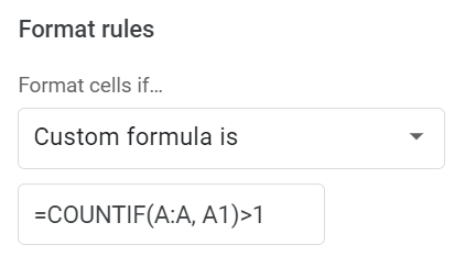
STEP 3: Under Format rules in the Format cells if… dropdown select and enter the formula you've developed for your specific situation:
STEP 4: Choose your desired Formatting style and click Done:

Your duplicates will be highlighted:
| A | |
| 1 | Salespeople |
| 2 | Michael |
| 3 | Jim |
| 4 | Dwight |
| 5 | Stanley |
| 6 | Jim |
| 7 | Phyllis |
| 8 | Andy |
Highlighting Duplicates In One Column Excluding The First Instance
Highlighting the second and subsequent instances of a duplicate can be useful to help remove duplicates while keeping one entry.
This requires a slight tweak to the range reference of the formula from above.
Here's the example again:
| A | B | C | |
| 1 | Salespeople | Formula | Output |
| 2 | Michael | =COUNTIF(A2:A8, A2)>1 | FALSE |
| 3 | Jim | =COUNTIF(A2:A8, A3)>1 | TRUE |
| 4 | Dwight | =COUNTIF(A2:A8, A4)>1 | FALSE |
| 5 | Stanley | =COUNTIF(A2:A8, A5)>1 | FALSE |
| 6 | Jim | =COUNTIF(A2:A8, A6)>1 | TRUE |
| 7 | Phyllis | =COUNTIF(A2:A8, A7)>1 | FALSE |
| 8 | Andy | =COUNTIF(A2:A8, A8)>1 | FALSE |
This time you only want the second 'Jim' in row 6 to be highlighted (so only this formula should output TRUE).
This can be done by adjusting the range referenced in each COUNTIF function so that it refers only to the current and previous rows, not the subsequent rows.
This way, when the first instance is encountered the COUNTIF output will be 1 and when the second is encountered it will be 2.
Here's what that looks like:
| A | B | C | |
| 1 | Salespeople | Formula | Output |
| 2 | Michael | =COUNTIF(A2, A2)>1 | FALSE |
| 3 | Jim | =COUNTIF(A2:A3, A3)>1 | FALSE |
| 4 | Dwight | =COUNTIF(A2:A4, A4)>1 | FALSE |
| 5 | Stanley | =COUNTIF(A2:A5, A5)>1 | FALSE |
| 6 | Jim | =COUNTIF(A2:A6, A6)>1 | TRUE |
| 7 | Phyllis | =COUNTIF(A2:A7, A7)>1 | FALSE |
| 8 | Andy | =COUNTIF(A2:A8, A8)>1 | FALSE |
Now you need to amend the top-left formula so that when it is auto-filled into the other cells by your conditional formatting it matches the other formulas.
The first formula is:
In a formula the cell reference A2 is the same as the range reference A2:A2.
You can re-write this formula based on this tip:
Now you want the first cell in the range reference to remain as A2 while the second changes to match the current row.
Absolute referencing can achieve this:
If you wanted to do an entire column, simply change the A2 references to A1 (the top-left most cell):
Remember to change the column references to suit your needs.
For example, if you need to highlight in column B the formula would need to change to:
Now enter this formula into a conditional formatting custom formula rule by following the instructions previously provided.


FREE RESOURCE
Google Sheets Cheat Sheet
12 exclusive tips to make user-friendly sheets from today:

You'll get updates from me with an easy-to-find "unsubscribe" link.
Highlighting Duplicates In Multiple Columns In Google Sheets
Here's some data:
| A | B | |
| 1 | First name | Last name |
| 2 | Michael | Scott |
| 3 | Jim | Halpert |
| 4 | Dwight | Schrute |
| 5 | Stanley | Hudson |
| 6 | Jim | Nixon |
| 7 | Phyllis | Vance |
| 8 | Jim | Halpert |
| 9 | Pam | Halpert |
| 10 |
The duplicate is 'Jim Halpert' in rows 3 and 8 but you can't rely on only the first name or last name as 'Jim Nixon' or 'Pam Halpert' would be highlighted incorrectly.
To highlight the duplicate correctly you need to combine the columns and then compare them:
| A | B | C | D | |
| 1 | First name | Last name | Formula | Output |
| 2 | Michael | Scott | =ArrayFormula(COUNTIF(A:A&B:B,A2&B2)>1) | FALSE |
| 3 | Jim | Halpert | =ArrayFormula(COUNTIF(A:A&B:B,A3&B3)>1) | TRUE |
| 4 | Dwight | Schrute | =ArrayFormula(COUNTIF(A:A&B:B,A4&B4)>1) | FALSE |
| 5 | Stanley | Hudson | =ArrayFormula(COUNTIF(A:A&B:B,A5&B5)>1) | FALSE |
| 6 | Jim | Nixon | =ArrayFormula(COUNTIF(A:A&B:B,A6&B6)>1) | FALSE |
| 7 | Phyllis | Vance | =ArrayFormula(COUNTIF(A:A&B:B,A7&B7)>1) | FALSE |
| 8 | Jim | Halpert | =ArrayFormula(COUNTIF(A:A&B:B,A8&B8)>1) | TRUE |
| 9 | Pam | Halpert | =ArrayFormula(COUNTIF(A:A&B:B,A9&B9)>1) | FALSE |
| =ArrayFormula(COUNTIF(A:A&B:B,A10&B10)>1) | TRUE |
The COUNTIF function doesn't ordinarily accept arrays (like A:A&B:B) as a range.
As such, you will need to wrap your formula in an ArrayFormula function to make it work properly.
There are two problems with this formula:
- The comparison is error-prone
- Blank rows are outputting TRUE
Fixing The Comparison
When you concatenate text with the & operator the text is merged without a delimiter.
"Michael" and "Scott" becomes "MichaelScott".
However, "Mic" and "haelScott" also becomes "MichaelScott".
You need something in between so that these things are recognised as being different.
When I need to do this I like to use rare characters like ¦.
You probably haven't seen this character before because it almost never appears in text. That makes it perfect for delimiting text.
If you change your formula slightly to be:
The error above can't happen as the outputs would now be "Michael¦Scott" and "Mic¦haelScott" which are different.
Adding this in you get:
| A | B | C | D | |
| 1 | First name | Last name | Formula | Output |
| 2 | Michael | Scott | =ArrayFormula(COUNTIF(A:A&"¦"&B:B,A2&"¦"&B2)>1) | FALSE |
| 3 | Jim | Halpert | =ArrayFormula(COUNTIF(A:A&"¦"&B:B,A3&"¦"&B3)>1) | TRUE |
| 4 | Dwight | Schrute | =ArrayFormula(COUNTIF(A:A&"¦"&B:B,A4&"¦"&B4)>1) | FALSE |
| 5 | Stanley | Hudson | =ArrayFormula(COUNTIF(A:A&"¦"&B:B,A5&"¦"&B5)>1) | FALSE |
| 6 | Jim | Nixon | =ArrayFormula(COUNTIF(A:A&"¦"&B:B,A6&"¦"&B6)>1) | FALSE |
| 7 | Phyllis | Vance | =ArrayFormula(COUNTIF(A:A&"¦"&B:B,A7&"¦"&B7)>1) | FALSE |
| 8 | Jim | Halpert | =ArrayFormula(COUNTIF(A:A&"¦"&B:B,A8&"¦"&B8)>1) | TRUE |
| 9 | Pam | Halpert | =ArrayFormula(COUNTIF(A:A&"¦"&B:B,A9&"¦"&B9)>1) | FALSE |
| 10 | =ArrayFormula(COUNTIF(A:A&"¦"&B:B,A10&"¦"&B10)>1) | TRUE |
Fixing The Blank Rows
Adding a simple IF statement to output FALSE if the row is completely blank will fix this issue:
Now you have a usable formula, you need to consider the relative and absolute referencing.
Remember that you'll want the conditional formatting to highlight across columns so you need to think about how your top-left formula will change as it moves down rows AND across columns.
Here's is the top-left formula for the range (the two columns):
You want the A1 and B1 references to be absolute for the column and relative for the row:
You want the A:A and B:B references to be absolute for the column:
Which makes the final formula:
Adding columns to this formula is a bit of a pain as many columns will result in a long formula.
Adding one column looks like this:
Adding two columns looks like this:
You get the idea, it's annoying to do for wide data.
If you're interested in a formula that's easier to add and remove columns from I came up with this while developing this post:
I don't think it's great to use because it's:
- too complicated to efficiently edit (or understand)
- far more computationally taxing on your sheet (will slow it down)
However, it is far easier to update as you only need to change the four range references.
To add conditional formatting based on this custom formula follow the instructions previously provided making sure to select multiple columns in STEP 1.
Highlighting Duplicates In Multiple Columns Excluding The First Instance
Highlighting the second and subsequent instances of a duplicate helps to find and remove duplicates while keeping the first entry.
Doing so requires a small change to the range array of the previous formula to make sure the COUNTIF is only acting on the current and previous rows, not the next rows:
The idea behind this is explained in greater detail here.
To add conditional formatting based on this custom formula follow the instructions previously provided making sure to select multiple columns in STEP 1.
FREE RESOURCE
Google Sheets Cheat Sheet
12 exclusive tips to make user-friendly sheets from today:
You'll get updates from me with an easy-to-find "unsubscribe" link.

![TRIM Google Sheets Function [With Quiz]](https://kierandixon.com/wp-content/uploads/trim-function-google-sheets.png)