How To Freeze Rows & Columns In Google Sheets

Kieran Dixon

Updated: March 3, 2021

To freeze: Click on the thick bars at the edge of the top-left corner of the sheet and drag them to where you need them. To unfreeze: Click and drag them back.

shows how to freeze and unfreeze rows and columns by clicking and dragging the thick bar at the top left of every sheet

Freezing rows and/or columns in Google Sheets means they remain visible as you scroll.

Why freeze rows and columns?

It makes your data more readable and therefore useful.

If you have a big data sets with lots of rows and columns it can be hard to understand if you don't freeze some rows and columns:

an example of how freezing rows and column in google sheets makes your data more readable and useful by keeping the frozen rows and columns visible as you scroll through a large data set

What would you like to do?

	A	B	C	D
1	ROWS		Freeze	Unfreeze
2	Desktop		View	View
3	Mobile	iOS	View	View
4	Mobile	Android	View	View
5	COLUMNS		Freeze	Unfreeze
6	Desktop		View	View
7	Mobile	iOS	View	View
8	Mobile	Android	View	View

Although the technical term for this process is 'freezing' rows or columns, people may also call it:

anchoring rows or columns
pinning rows or columns
making a sticky row or column
keeping top row visible (or first column)
freezing panes or the header

How To Freeze Rows In Google Sheets

Mouse click and drag (quickest and easiest)

This is my go-to method for freezing rows.

I think it's the best because you can freeze as many rows as you want in less than a second.

STEP 1: Move your mouse to the bottom edge of the box in the top left of the sheet. Your cursor will change into a tiny, open hand.

You don't have to do this using the box in the top left. It will work at any point along the bottom of the column labels.

STEP 2: Click your mouse and hold (the tiny hand will clench like it's grabbed something) then drag your mouse down.

STEP 3: A line will appear across your screen and move as you drag your mouse. When the line is where you'd like to freeze up to, release the mouse.

That's it! Your rows are now frozen.

Here's the drag and drop row freezing process in action:

freezing rows by dragging and dropping the freeze line in google sheets

This is great because you can choose how many rows to freeze as you're doing it.

Once the freeze is in place you can easily change it by following the same steps, this time clicking and dragging the already established freeze line:

how to change the number of frozen rows when one or more is already frozen in google sheets

View Menu

You can also use the View menu to freeze rows in Google Sheets.

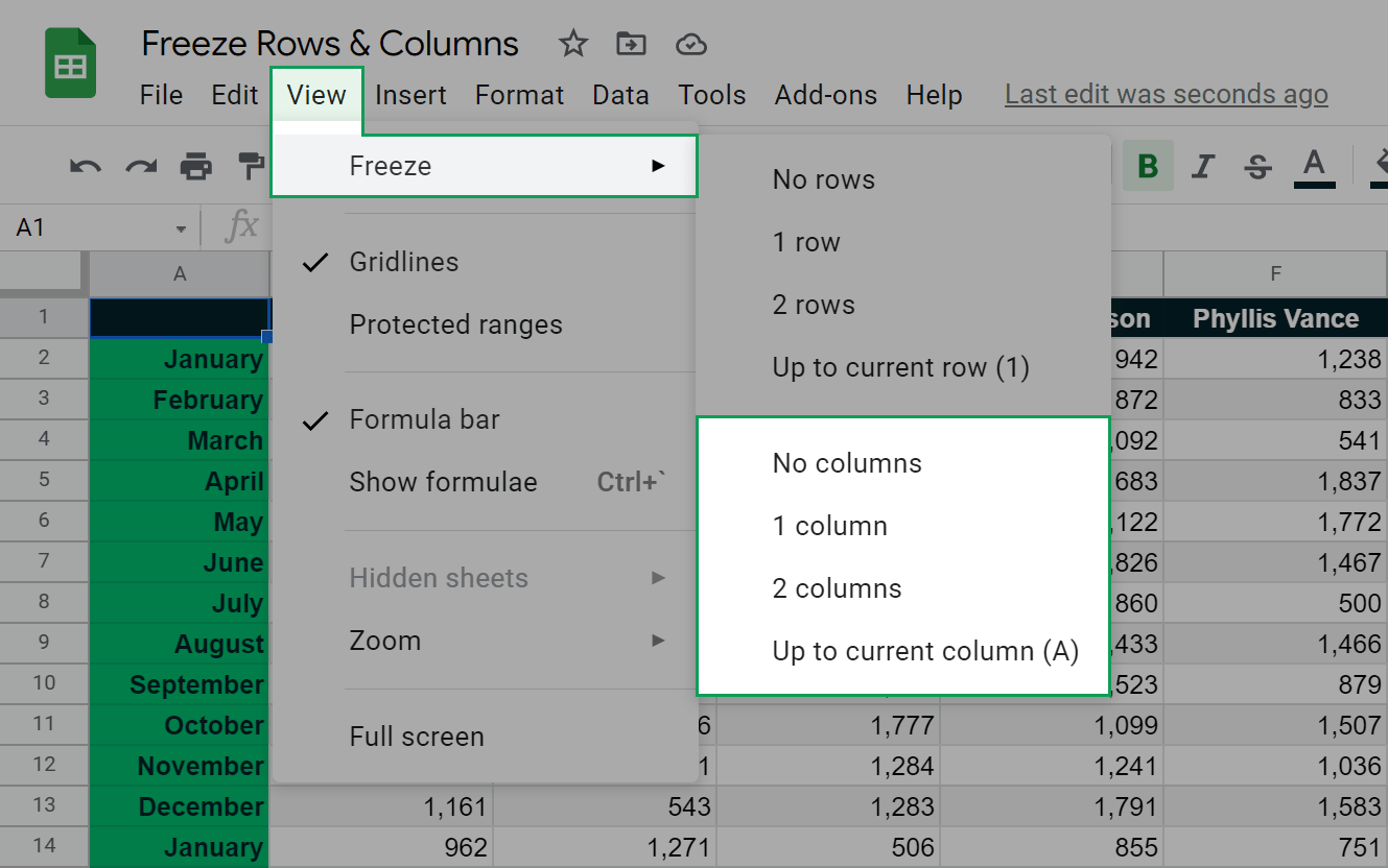
STEP 1: Click on the View menu item, hover over Freeze in the dropdown and in the menu that appears, click on either 1 row, 2 rows, or Up to current row:

location of the view menu that allows you to freeze rows in google sheets

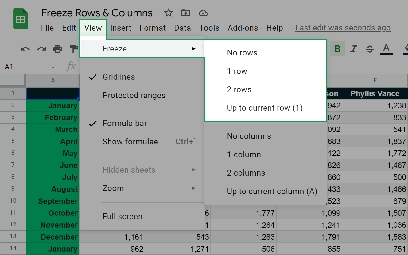
Your rows are now frozen.

Here's the View menu row freezing process in action:

using the view menu to freeze one or multiple rows in google sheets

If you want to freeze more than two rows using this method you first need to select a cell in the last row you want frozen.

Keyboard shortcuts

There are also keyboard shortcuts you can use to freeze rows in Google Sheets.

I don't use these shortcuts myself because the click and drag method above is so easy.

However, some spreadsheet users hates touching the mouse so here they are:

	A	B	C
1	Action	Shortcut
2	Action	*Windows, Chrome OS*	*Mac*
3	Freeze 1 row	Alt + W, F, R<br>Alt + V, R, O	None
4	Freeze 2 rows	Alt + V, R, W	None
5	Freeze up to current row	Alt + V, R, U	None

This is what using the shortcuts looks like (on Windows):

freezing rows using keyboard shortcuts in google sheets

FREE RESOURCE

Google Sheets Cheat Sheet

12 exclusive tips to make user-friendly sheets from today:

You'll get updates from me with an easy-to-find "unsubscribe" link.

How To Unfreeze Rows In Google Sheets

Your sheet has frozen rows but you don't want them. Here's three ways to fix this:

Mouse click and drag

STEP 1: Move your mouse to the already established freeze line. Your cursor will change into a tiny, open hand.

STEP 2: Click your mouse and hold (the tiny hand will clench like it's grabbed something) then drag your mouse up to the column labels.

This method works at any point across the established freeze line.

STEP 3: A line will appear across your screen and move as you drag your mouse. When the line is level with the bottom of the column labels, release the mouse.

That's it! Your rows are no longer frozen.

Here's the drag and drop row unfreezing process in action:

unfreezing rows by dragging and dropping the existing frozen row line

View Menu

You can also use the View menu to unfreeze rows in Google Sheets.

STEP 1: Click on the View menu item, hover over Freeze in the dropdown and in the menu that appears, click on No rows:

location of the view menu that allows you to unfreeze rows in google sheets

Your rows are now unfrozen.

Here's the View menu row unfreezing process in action:

unfreezing rows using the view menu in google sheets

Keyboard shortcut

There is a keyboard shortcut to unfreeze rows in Google Sheets:

	A	B	C
1	Action	Shortcut
2	Action	*Windows, Chrome OS*	*Mac*
3	Unfreeze rows	Alt + V, R, R	None

This is what using the shortcut looks like (on Windows):

unfreezing rows using a keyboard shortcut in google sheets

How To Freeze Columns In Google Sheets

Mouse click and drag (quickest and easiest)

This is my go-to method for freezing columns.

I think it's the best because you can freeze as many columns as you want in less than a second.

STEP 1: Move your mouse to the right edge of the box in the top left of the sheet. Your cursor will change into a tiny, open hand.

You don't have to do this using the box in the top left. It will work at any point along the right edge of the row labels.

STEP 2: Click your mouse and hold (the tiny hand will clench like it's grabbed something) then drag your mouse to the right.

STEP 3: A vertical line will appear on your screen and move as you drag your mouse. When the line is where you'd like to freeze up to, release the mouse.

That's it! Your columns are now frozen.

Here's the drag and drop column freezing process in action:

freezing columns by dragging and dropping the freeze line in google sheets

This is great because you can choose how many columns to freeze as you're doing it.

Once the freeze is in place you can easily change it by following the same steps, this time clicking and dragging the already established freeze line:

how to change the number of frozen columns when one or more is already frozen in google sheets

View Menu

You can also use the View menu to freeze columns in Google Sheets.

STEP 1: Click on the View menu item, hover over Freeze in the dropdown and in the menu that appears, click on either 1 column, 2 columns, or Up to current column:

location of the view menu that allows you to freeze columns in google sheets

Your columns are now frozen.

Here's the View menu column freezing process in action:

using the view menu to freeze one or multiple columns in google sheets

If you want to freeze more than two columns using this method you first need to select a cell in the last (rightmost) column you want frozen.

Keyboard shortcuts

There are also keyboard shortcuts you can use to freeze columns in Google Sheets.

I don't use these shortcuts myself because the click and drag method above is so easy.

However, some spreadsheet users hates touching the mouse so here they are:

	A	B	C
1	Action	Shortcut
2	Action	*Windows, Chrome OS*	*Mac*
3	Freeze 1 column	Alt + W, F, C<br>Alt + V, R, L	None
4	Freeze 2 columns	Alt + V, R, M	None
5	Freeze up to current column	Alt + V, R, P	None

This is what using the shortcuts looks like (on Windows):

freezing columns using keyboard shortcuts in google sheets

How To Unfreeze Columns In Google Sheets

Your sheet has frozen columns but you don't want them. Here's three ways to fix this:

Mouse click and drag

STEP 1: Move your mouse to the already established freeze line. Your cursor will change into a tiny, open hand.

STEP 2: Click your mouse and hold (the tiny hand will clench like it's grabbed something) then drag your mouse left to the row labels.

This method works at any point across the established freeze line.

STEP 3: A vertical line will appear across your screen and move as you drag your mouse. When the line is level with the right edge of the row labels, release the mouse.

That's it! Your columns are no longer frozen.

Here's the drag and drop column unfreezing process in action:

unfreezing columns by dragging and dropping the existing frozen row line

View Menu

You can also use the View menu to unfreeze columns in Google Sheets.

STEP 1: Click on the View menu item, hover over Freeze in the dropdown and in the menu that appears, click on No columns:

location of the view menu that allows you to unfreeze columns in google sheets

Your rows are now unfrozen.

Here's the View menu column unfreezing process in action:

Keyboard shortcut

There is a keyboard shortcut to unfreeze columns in Google Sheets:

	A	B	C
1	Action	Shortcut
2	Action	*Windows, Chrome OS*	*Mac*
3	Unfreeze columns	Alt + V, R, C	None

This is what using the shortcut looks like (on Windows):