How To Create A Dropdown List In Google Sheets

Kieran Dixon Updated:  June 3, 2021

Dropdowns in Google Sheets make your spreadsheets user-friendly.

They help to prevent formula and script errors by making sure that data is entered exactly as you need it to be.

Wait... why am I trying to convince you? You already know they're awesome.

You're here to make them:

• Create a dropdown
• Edit a dropdown
• Color code a dropdown
• Copy a dropdown
• Remove a dropdown

How To Create Dropdown Lists In Google Sheets

Not on desktop? Click for mobile instructions: iPhone/iPad and Android.

STEP 1: Select the cell/s you want to contain your dropdown list by clicking (to select a single cell) and dragging (to select a range). Selected cells are highlighted and bordered in blue.

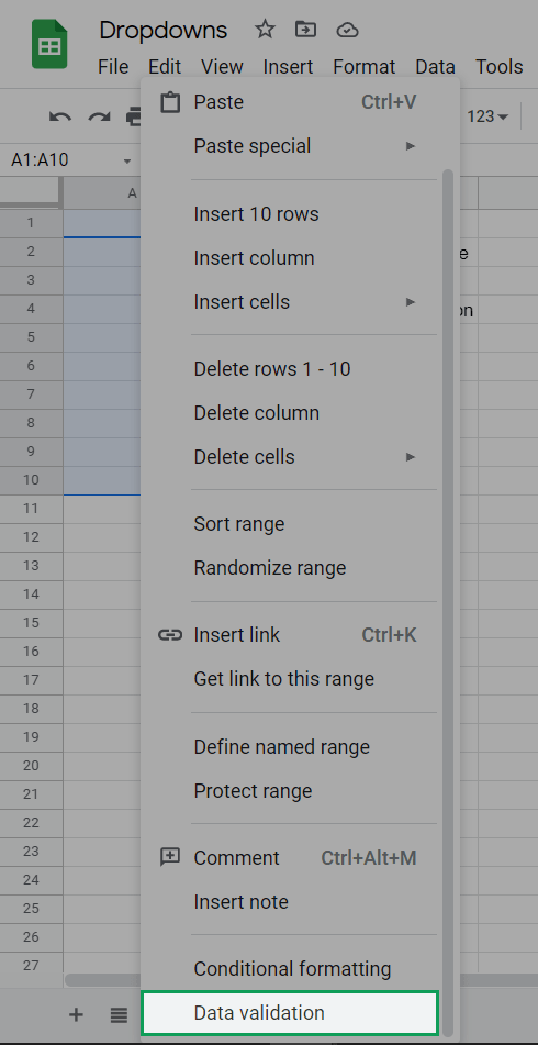
STEP 2: Click on the Data menu item and click on the Data validation option:

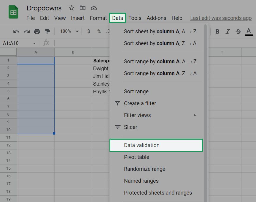
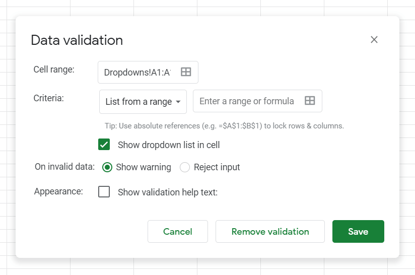
You'll now see the Data validation popup:

You can also access this menu by right-clicking on your selection and choosing the Data validation option for the list that appears:

Or using one of these keyboard shortcuts (on Windows):

Alt + A, V or Alt + D, L or Alt + D, V

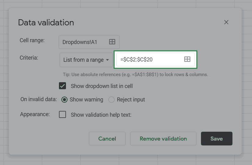
Let's talk through the popup options:

Cell range:

Here you can confirm which cell/s you want to contain the dropdown list.

If you've already made your selection properly you can leave this.

If you need to make a change, type in the correct range or click on the 'Select data range' icon and make a new selection:

Criteria:

This is where the options in your dropdown are chosen.

From the dropdown menu here, only 'List from a range' and 'List of items' are relevant when creating a dropdown:

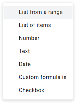
List from a range

This is my preferred method for creating dropdown lists.

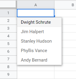
You select a range from within your sheet that contains the items you want in your dropdown and Google Sheets automatically gets only the unique entries and puts them in your dropdown:

Better yet, you can expand the range beyond your current list to allow for future entries:

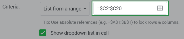
To save time in having to highlight the entire column you can simply remove the numbers from the last column reference (C2:C instead of C2:C20):

This will select all the way down to the last cell of that column, meaning all future updates to the dropdown list will be captured.

The blank cells in the range are simply ignored.

When you select a range Google Sheets assumes that you want it to be referenced absolutely (e.g. $A$1:$B$1). This means that if you copy and paste or autofill the dropdown elsewhere in the spreadsheet the dropdown list will be created from the same range.

In fact, if you make a selection, save it, and open the data validation again the range you selected will automatically have absolute referencing applied to it:

If you want the reference to be partially or completely relative (e.g. $A1:$B1, A$1:B$1, or A1:B1) you need to specify the type of referencing using dollar signs in the 'Enter a range or formula' text box:

If you choose relative references and copy and paste or autofill, the dropdown will reference a range equivalent to the relative movement that occurred during the copy and paste or autofill:

The newly created dropdown is no longer referencing $C2:$C20. The relative reference means that instead it is referencing $C3:$C21, excluding Dwight Schrute from the dropdown.

The range you select doesn't have to be in the same sheet as your dropdown list.

I usually include a Settings sheet in my Google Sheets. Among other things, this is where I will put my dropdown list options so they are all in one place.

When selecting the range you simply click to the other sheet and make your selection there:

Using a list from a range makes your dropdowns far more flexible by allowing you to edit many dropdowns in different parts of your sheet from a single location:

With a 'List of items' (below) you have to update non-adjacent dropdowns in multiple locations individually.

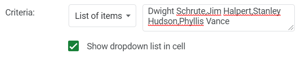
List of items

Type in the list of items you want to appear in your dropdown separated by a comma:

When entering your list you can add line breaks for clarity. This will have no effect on the output of the dropdown (and they won't be there when you edit it again):

I would only use the 'List of items' option with dropdowns that contain two opposite choices (e.g. Yes or No).

Even then, I would avoid it.

You never know how a sheet is going to change in the future and hard-coding values is generally bad practice.

Let's look at an example:

You have two identical 'List of items' dropdowns that list salespeople in separate locations within the sheet:

A new salesperson joins the team. You update the first dropdowns but the other doesn't update:

You now have to add the salesperson to each dropdown (if they aren't adjacent and can be included in a single selection).

Using a 'List from a range' dropdown allows for updates to all dropdowns at once.

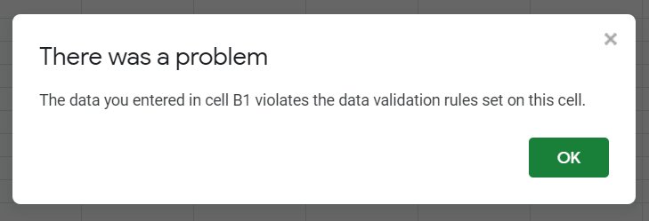
On invalid data:

You have two options:

Show warning

This option tells the user that the value they've entered isn't one of the dropdown options but still allows them to enter it:

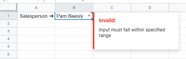
Reject input

This option tells the user that they aren't allowed to enter a value that isn't one of the dropdown options:

It might seem like a harsh user experience but this is my go-to option.

Spreadsheets aren't like normal software applications that are hard for users to break.

Spreadsheets are fickle and I love protecting my formulas and scripts from unforeseen errors by limiting user input.

Appearance:

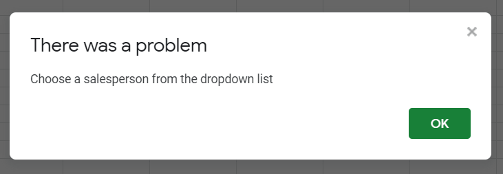
You can tick a checkbox to show or not show validation help text when an input is rejected.

If you choose to show it, you have control over the message that users see:

I like to write a unique and descriptive message that tells the user exactly what they need to do to satisfy the data validation:

This help text will appear instead of the default text if you've chosen to reject invalid inputs:

When you're happy with all of these options, click the 'Save' button and voila!

You have yourself a working dropdown list:

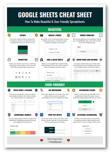
FREE RESOURCE

Google Sheets Cheat Sheet

12 exclusive tips to make user-friendly sheets from today:

Get The Cheat Sheet ➜

You'll get updates from me with an easy-to-find "unsubscribe" link.

How To Edit Dropdown Lists In Google Sheets

STEP 1: Select the dropdown/s you want to edit.

STEP 2: Open the Data validation popup using either:

1. Data in the top menu ➜ Click the Data validation option
2. Right click and choose the Data validation option
3. One of these keyboard shortcuts (Windows only): Alt + A, V or Alt + D, L or Alt + D, V

STEP 3: Change the cell range, criteria, invalid data, or help text options as required.

If you created your dropdown list from a range that included room for additional options you can add or remove options by editing the data in that range:

How To Color Code Dropdown Lists In Google Sheets

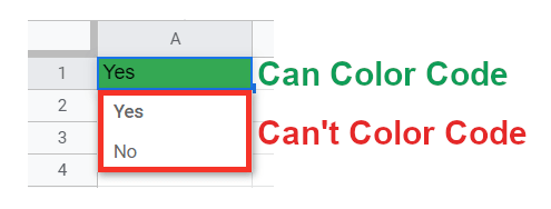
In Google Sheets you can't color the actual items when they're in the dropdown list.

What you can color is the options once they're in the cell:

This color coding is achieved using conditional formatting.

Conditional formatting is a big topic that I'm only going to touch on here to help you achieve this one effect.

STEP 1: Select the dropdown/s you want to color code.

STEP 2: Open the conditional formatting sidebar using one of the following methods:

1. 'Format' in the top menu ➜ Click the 'Conditional formatting' option
2. Right click and choose the 'Conditional formatting' option
3. The keyboard shortcut Alt + H, L (only on Windows)

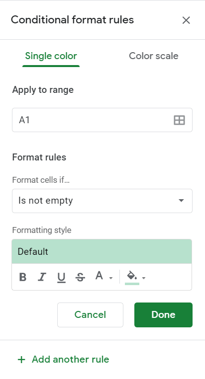
STEP 3: Add a new rule to your selection by editing the 'Format rules':

You can trigger the formatting using the 'Format cells if…' dropdown:

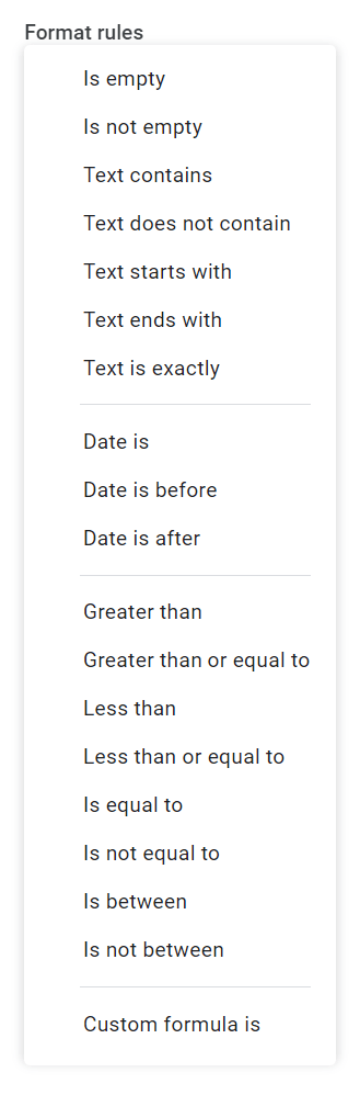
All except the Custom formula is option are self-explanatory. I'm not going to address that now because that functionality is more complicated than we need it to be.

Choose the most relevant option for your situation and additional inputs will be required.

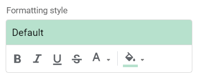
You can then choose the Formatting style you want to be applied when the rule is met:

When you're happy, click the 'Done' button and you're good to go!

Let's work through an example:

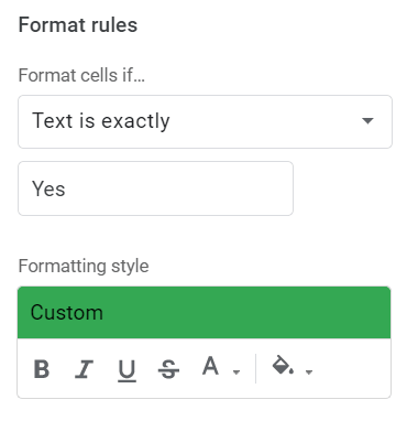
I want a dropdown to be green if 'Yes' and red if 'No'.

I'll need two conditional formatting rules to make this work, one for green and one for red.

With the correct range selected I make the following Text is exactly rule and formatting:

Then repeat this process with red formatting for 'No':

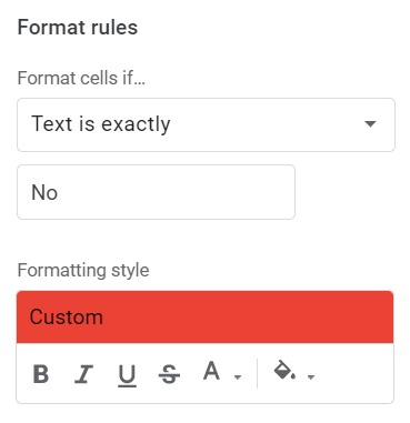
And you end up with a color-coded dropdown:

How To Copy Dropdown Lists In Google Sheets

STEP 1: Select the dropdown/s you want and copy using:

1. The keyboard shortcut Ctrl + C or ⌘ + C
2. Edit in the top menu ➜ Click the Copy option
3. Right click and choose the Copy option

STEP 2: Select where you want to paste the dropdown/s and paste using:

1. The keyboard shortcut Ctrl + V or ⌘ + V
2. Edit in the top menu ➜ Click the Paste option
3. Right click and choose the Paste option

This will paste with content and formatting:

If you want to paste the dropdown without the formatting and content you can copy it and then use a special paste:

1. The keyboard shortcut Alt + E, S, D (only on Windows with compatible shortcuts enabled)
2. Edit in the top menu ➜ Hover over the Paste special option ➜ Click the Paste data validation only option
3. Right click and hover over the Paste special option ➜ Click the Paste data validation only option

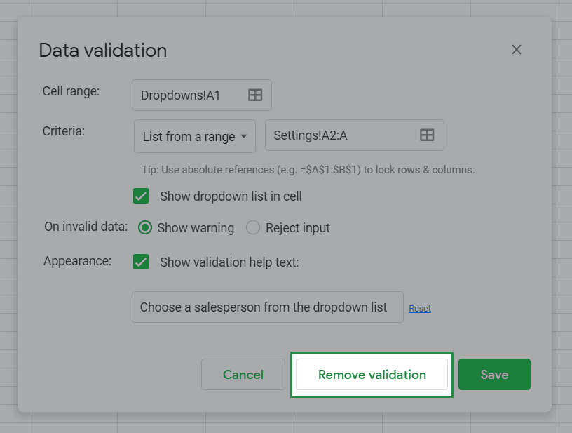
How To Remove Dropdown Lists In Google Sheets

STEP 1: Select the dropdown/s you want to remove.

STEP 2: Open the Data validation popup using either:

1. Data in the top menu ➜ Click the Data validation option
2. Right click and choose the Data validation option
3. One of these keyboard shortcuts (Windows only): Alt + A, V or Alt + D, L or Alt + D, V

STEP 3: Click the 'Remove validation' button:

A quick way to achieve this is to simply copy and paste (Ctrl + C or ⌘ + C then Ctrl + V or ⌘ + V) a cell that doesn't have a dropdown where the dropdown you want to remove is:

How To Create Dropdown Lists In The Google Sheets iPhone And iPad App

You can't.

It sucks, but currently the iPhone and iPad apps don't have this functionality.

When they do, I'll show you how.

You can use dropdown lists using the iPhone and iPad apps:

However, for the time being to create them you will need to use the desktop application.

How To Create Dropdown Lists In The Google Sheets Android App

Not creating? Click for instructions to edit or remove instead.

STEP 1: Select the cell/s in which you want to create a dropdown list by touching them.

STEP 2: Tap the stacked dots in the top right corner:

STEP 3: In the menu that appears, tap the Data validation option

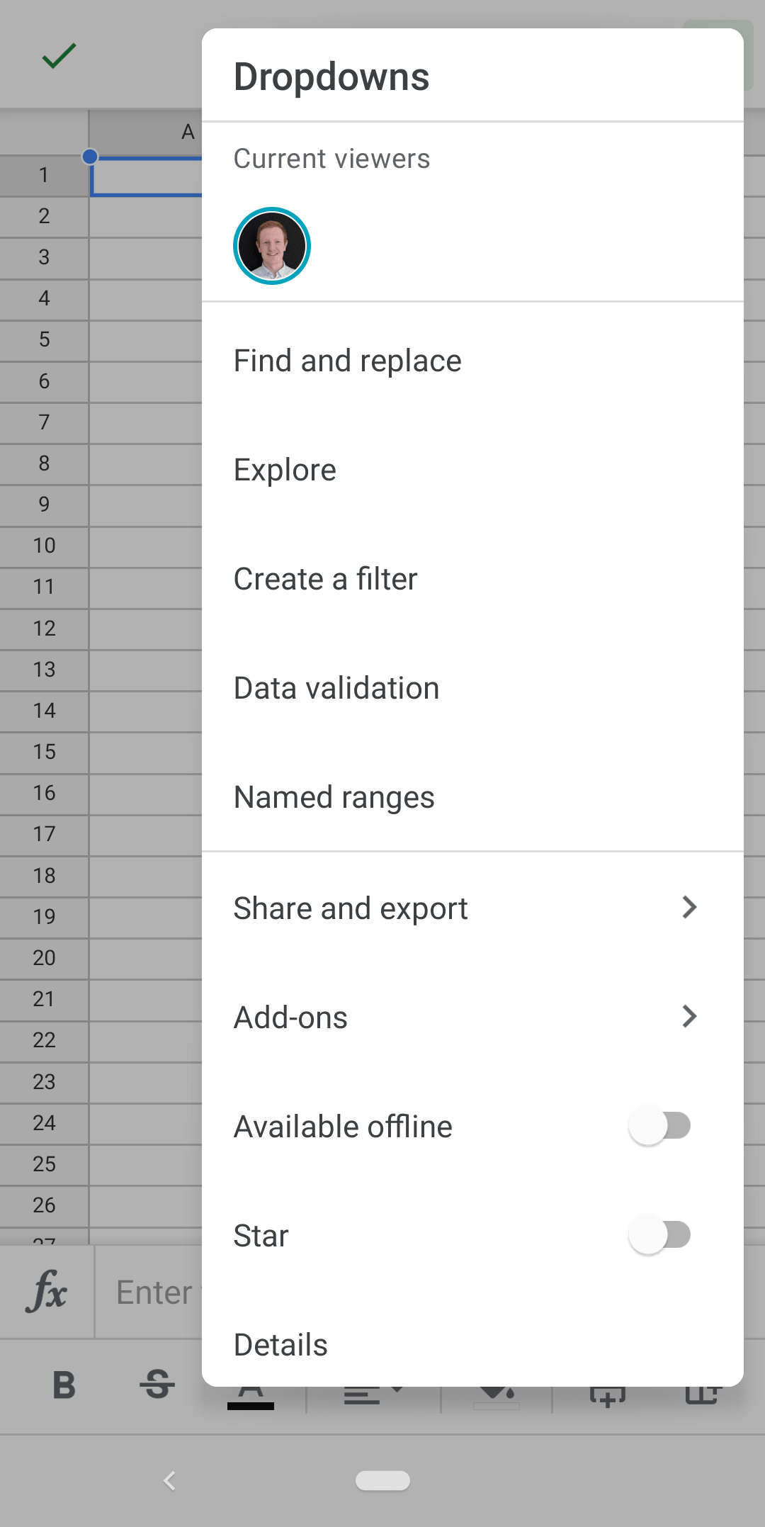
STEP 4: You can now see all of the options available to create, edit and remove a dropdown list:

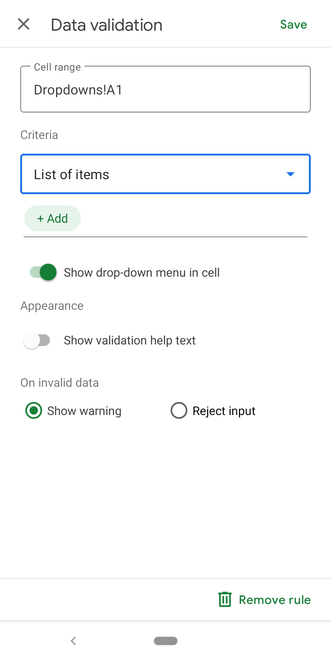
Cell range (on Android):

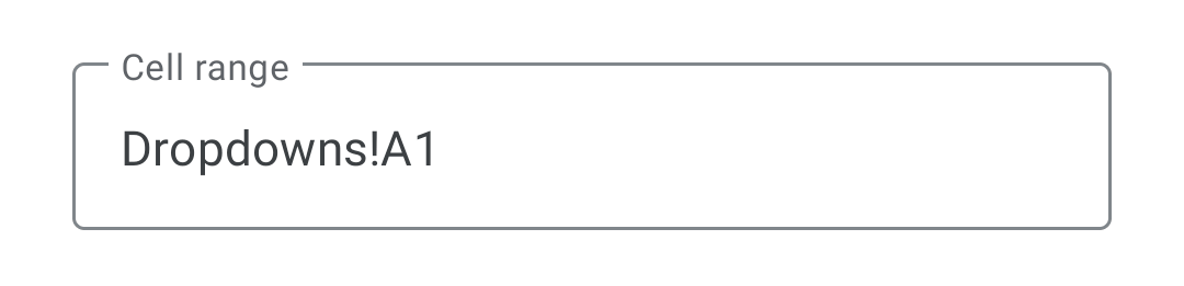
Type in the range you want to apply the dropdown to (if it doesn't already match the selection you made in STEP 1.

There is no option to select a different range without exiting this menu (which you can do on the desktop app).

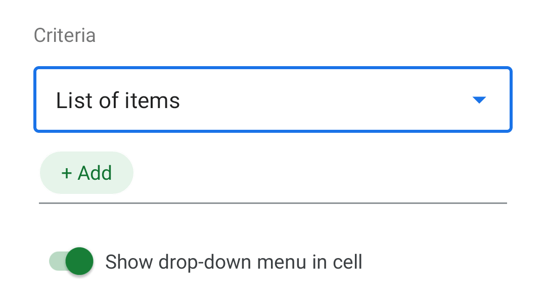
Criteria (on Android):

For a dropdown list choose either List of items or List from a range from the criteria options:

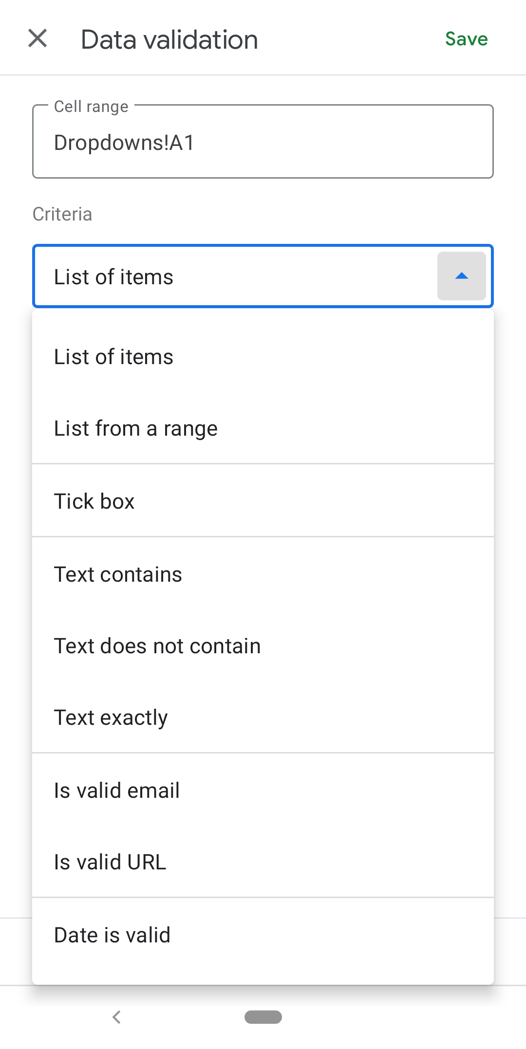
For either type of list to show a dropdown you must toggle the Show drop-down menu in cell option.

List of items (on Android)

Type in the items you want in your dropdown list:

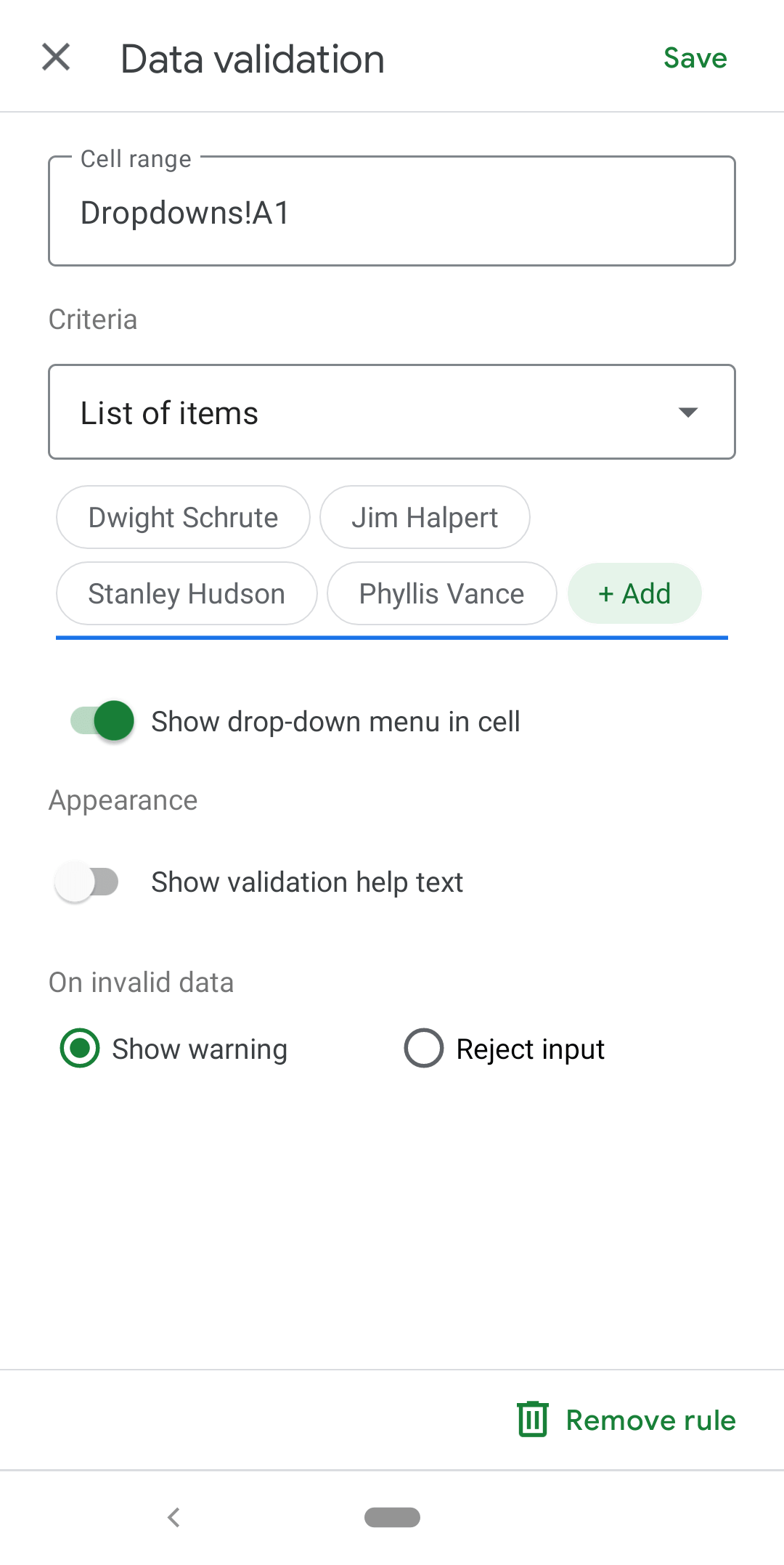
Here's what the whole process looks like:

List from a range (on Android)

Type in the range from your sheet where your dropdown options are listed:

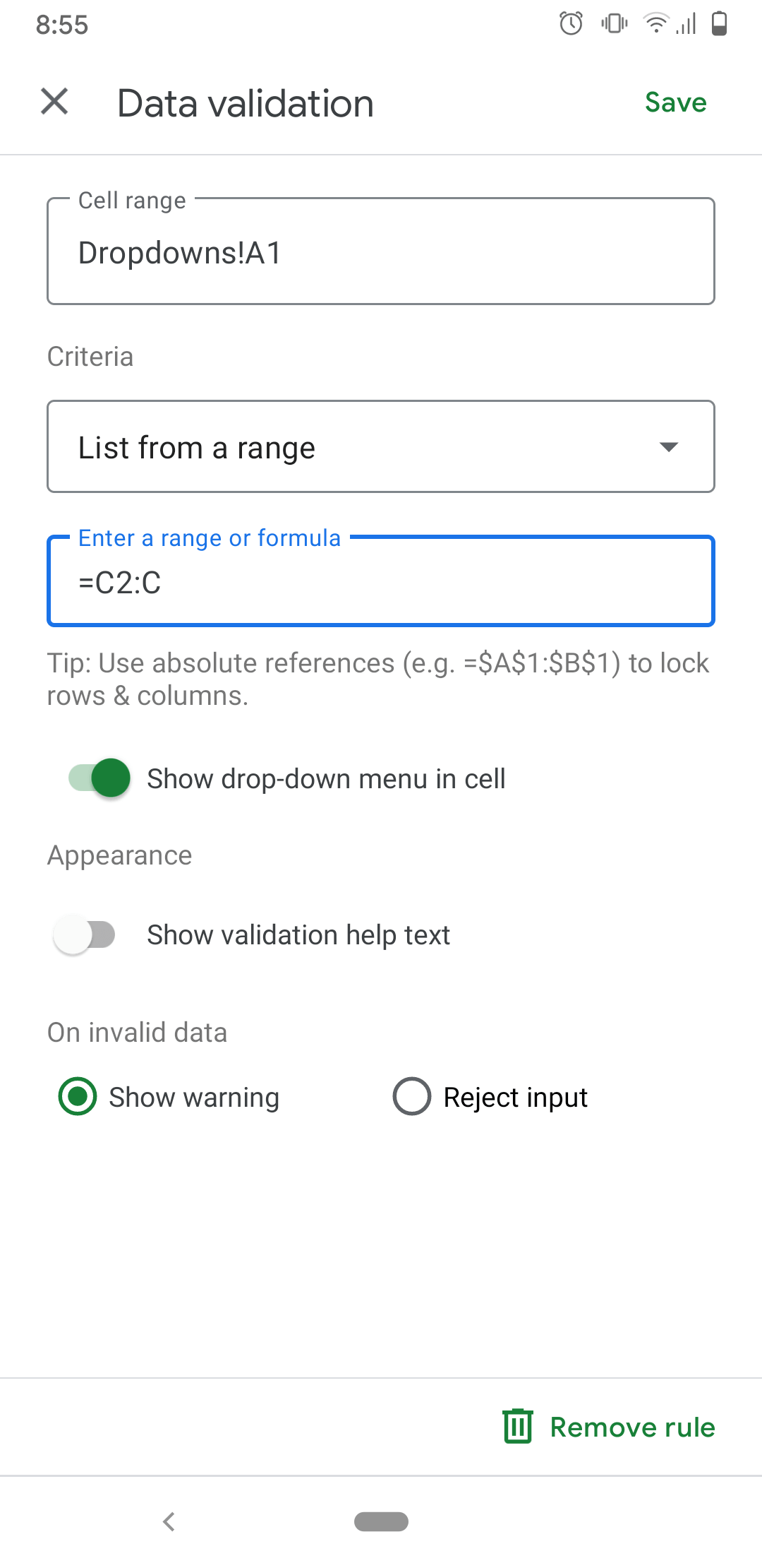
Here's what the whole process looks like:

Appearance (on Android)

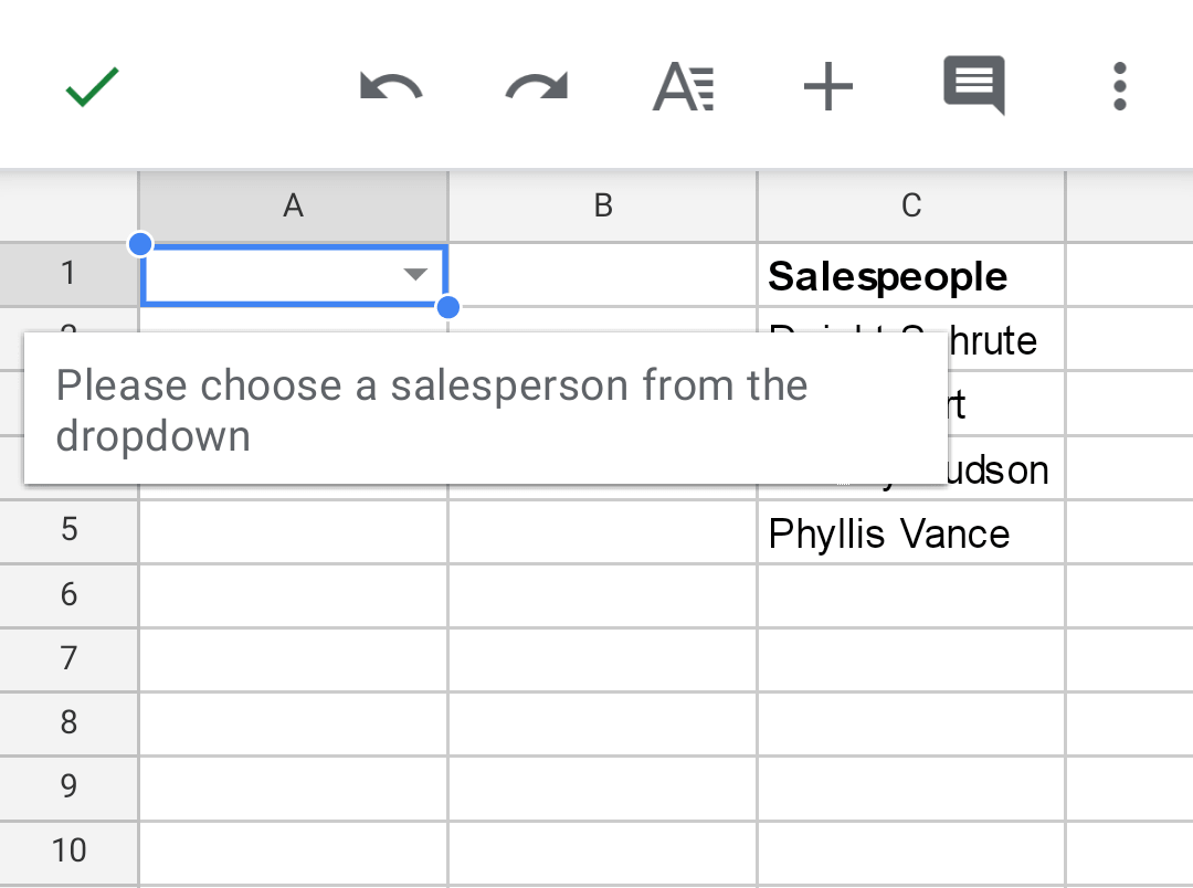
Toggle the Show validation help text option to type in a custom message:

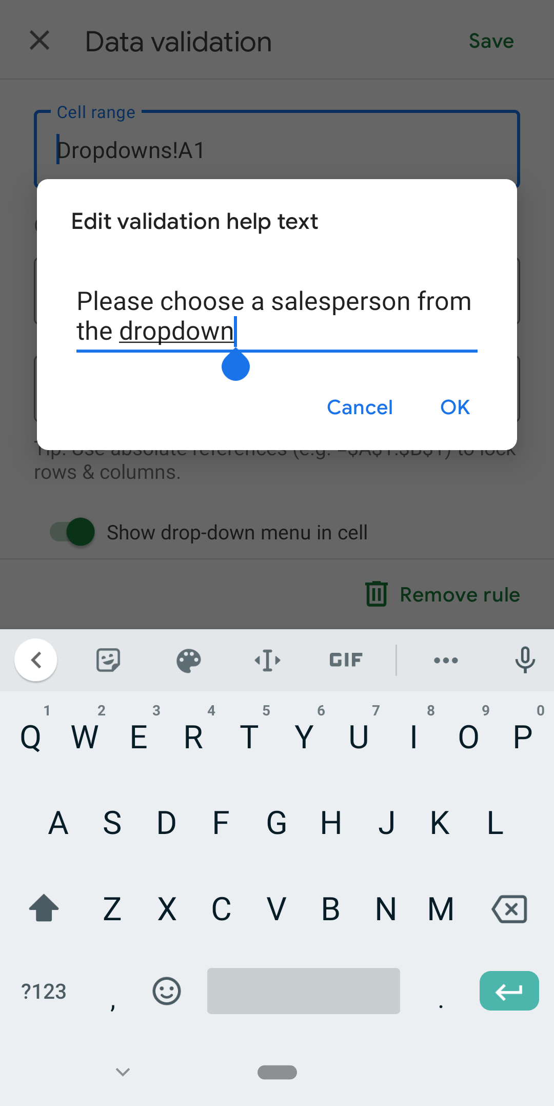
This message appears before a user enters data:

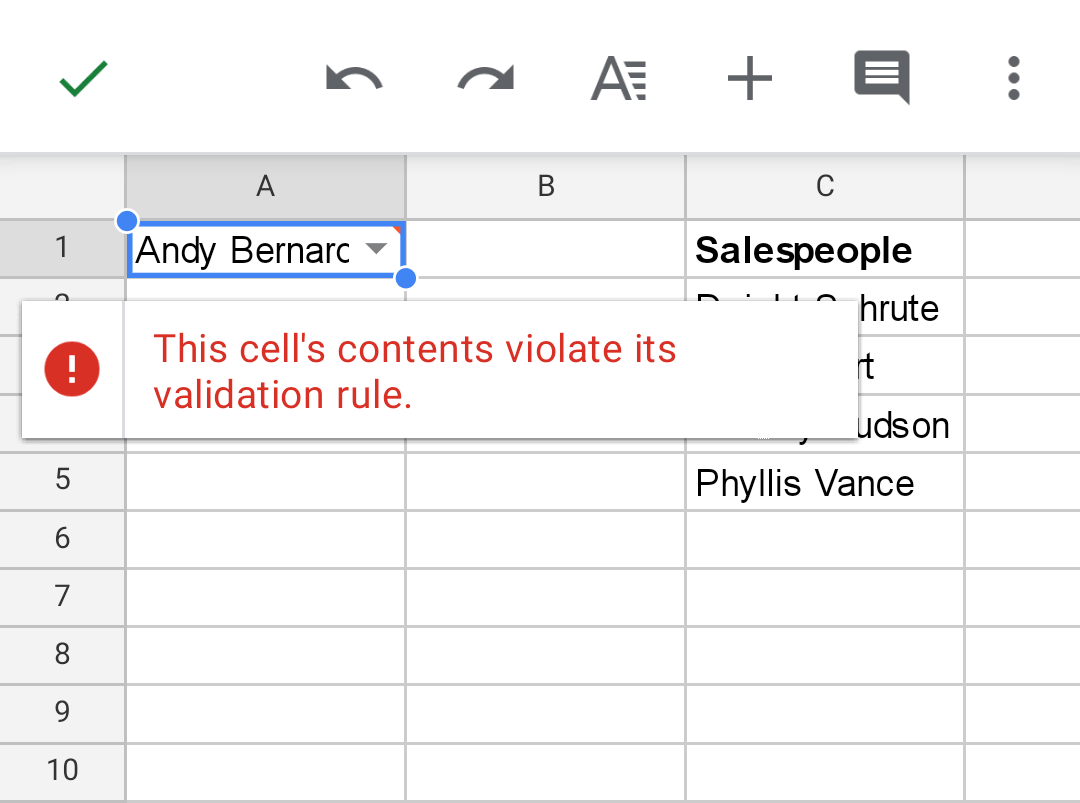
And if a user input does not match the data validation:

On invalid data (on Android)

Here you can choose whether to Show warning or Reject input when an entered value does not match one of the available dropdowns:

Showing a warning can be risky as the validation still accepts a user's input. This might cause unforeseen errors in formulas and scripts attached to the sheet.

This is what showing a warning looks like:

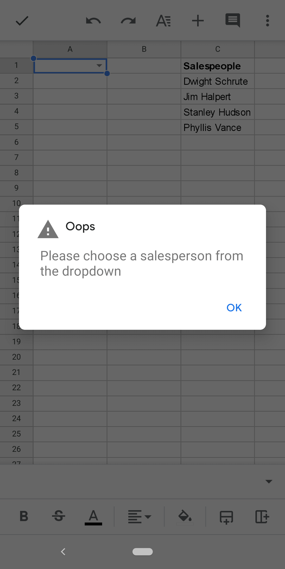
Rejecting the input is my preferred option as it guarantees the user can't enter data I haven't accounted for.

This is what it looks like (the custom message from above appears):

Editing a List of items on Android

To edit a List of items dropdown you simply need to open the Data validation menu using the steps above and amend the various options.

Here's a clip of adding an item to the dropdown list:

Editing a List from a range on Android

It's easy to edit a List from a range dropdown when they're created properly. You don't even need to open the Data validation menu.

First off, when you use a List from a range dropdown it's good practice to include a range that's larger than the existing list so you can easily add items in the future.

In the example above the chosen range was C2:C.

This means anything entered in column C will appear in the dropdown making it incredible easy to edit:

If you need to edit other aspects of the dropdown (e.g. warning message) simply select the dropdown and navigate to the Data validation menu using the steps outlined above.

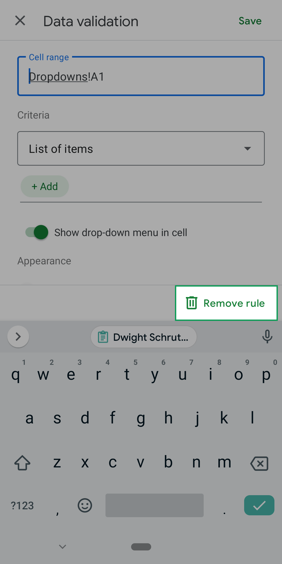
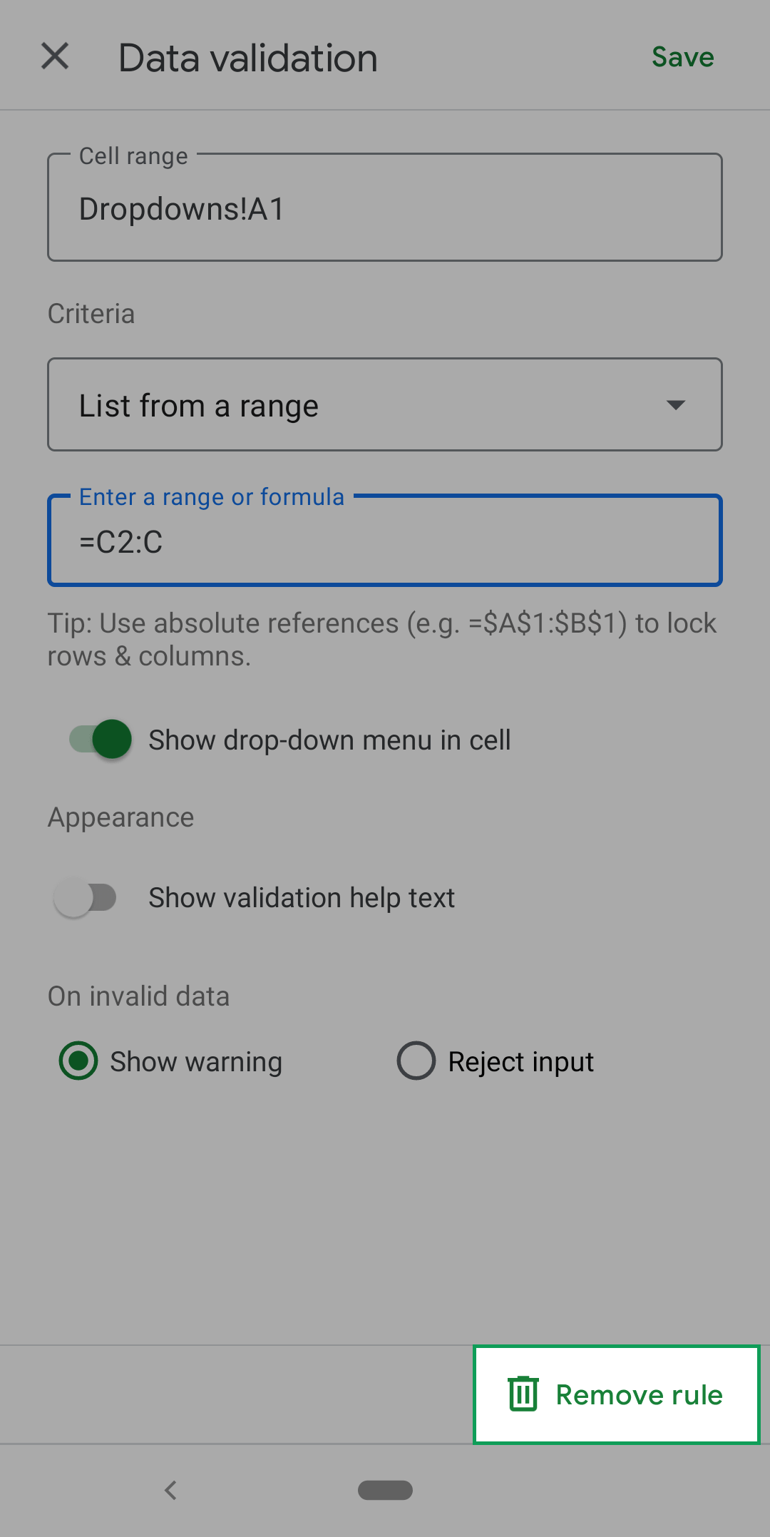
Remove a dropdown on Android

Select the dropdown and navigate to the Data validation menu using the steps outlined above.

Then tap on the Remove rule button here:

Or here:

Here a clip of the process:

FREE RESOURCE

Google Sheets Cheat Sheet

12 exclusive tips to make user-friendly sheets from today:

Get The Cheat Sheet ➜

You'll get updates from me with an easy-to-find "unsubscribe" link.

Kieran Dixon started using spreadsheets in 2010. He leveled-up his skills working for banks and running his own business. Now he makes Google Sheets and Apps Script more approachable for anyone looking to streamline their business and life.

You might like:

Radio Buttons In Google Sheets

Want radio buttons in Google Sheets? Here's a flexible, plug and play script that creates radio buttons in both rows and columns.

How To Add A Date Picker In Google Sheets

Need to add a date picker in Google Sheets? Here are step-by-step instructions for the desktop, iPhone, iPad, and Android apps.