Formula Parse Errors In Google Sheets & How To Fix Them
 Updated: December 16, 2021
 Formula parse errors in Google Sheets are frustrating.
That's why this page teaches you what each formula parse error is, why they happen and how to fix formula parse errors, and how to get rid of errors in Google Sheets by stopping them from being seen.
Find out how to fix your error by clicking on what you're seeing in Google Sheets (an error in a cell or the popup message below):
There was a problem
It looks like your formula has an error. If you don't want to enter a formula, begin your text with an apostrophe (').
OKErrors can be caused:
- Directly by the formula within that cell, or
- Indirectly when the formula in that cell references another cell that contains an error
#DIV/0!
You'll see this error when you try to divide by zero… because you can't divide by zero.
Here's a simple example:
Function DIVIDE parameter 2 cannot be zero.
The #DIV/0! error happens whenever you use a function (or operator) that involves division when the number to divide by (denominator) evaluates to zero (including when you provide a blank cell).
Here are just a few examples of functions that can create this error:
- DIVIDE
- QUOTIENT
- MOD
- AVERAGE
- AVERAGEIF
How To Fix A #DIV/0! Error
You need to find the zero (or blank cell/s) causing the error.
This is easy in simple formulas but more difficult in complex ones.
Here's a neat trick to help out.
When you're typing your formula you can highlight complete functions (including those with nested functions) to see a little tooltip that contains the output:
This only works when the output is a single text, number, or BOOLEAN value.
If the highlighted function outputs an array of values it won't be displayed.
When you find the guilty 0 (or blank cell), you can change it.
However, if the data is variable or you can't control it (e.g. it comes from a Google Form) you can account for the potential of a zero denominator with a function like IFERROR.
This function outputs the value if it isn't an error.
If the value is an error, it instead outputs the entered [value_if_error] or nothing (if omitted).
From the first example:
Would output "Can't divide by zero" instead of a #DIV/0! error.
This might not be an ideal solution in more complex formulas that could output more than one type of error.
For that, you might want to get more specific with your error handling using the ERROR.TYPE function which outputs 2 if its input results in a #DIV/0! error.


FREE RESOURCE
Google Sheets Cheat Sheet
12 exclusive tips to make user-friendly sheets from today:

You'll get updates from me with an easy-to-find "unsubscribe" link.
#ERROR!
You'll see this error when Google Sheets can't understand (parse) your formula.
It's trying to read it, but it just can't for some reason.
Here's something that can cause it:
Formula parse error.
Multiple arguments provided to the SUM function need to be separated by a comma. Without the comma, Google Sheets can't understand what it's supposed to do and throws the error.
#ERROR! doesn't happen with specific operators or functions but instead can happen in any formula.
It just takes one syntax error to ruin the whole thing.
Can you find the error in this formula?
How To Fix An #ERROR! Error
Go back over your formula and check each function to make sure you're not missing important syntax.
You're looking for missing (or unnecessary additional) syntax in between values, functions, and arguments in your formula.
Keep an eye out for:
- Parentheses ()
- Braces {}
- Colons :
- Ampersands &
- Commas ,
- Dollar signs $
- Percentage symbols %
You should find (and be able to fix) the problem by reviewing these things.
For those playing along: the formula above was missing an ampersand to concatenate the data points:
#N/A
The output you want is Not Available.
That's what #N/A means.
This error usually comes up when a function is looking something up and it isn't there.
Functions like VLOOKUP and MATCH search columns for specific data and when they can't find it, you get an #N/A error:
Did not find value 'search_key' in VLOOKUP evaluation.
Here's an example:
| A | B | C | D | E | |
| 1 | Salesperson | Sales | Search for | Formula | Output |
| 2 | Dwight | $10,000 | Stanley | =VLOOKUP(C2,$A$2:$B$6,2,0) | $8,000 |
| 3 | Jim | $9,000 | Pam | =VLOOKUP(C3,$A$2:$B$6,2,0) | #N/A |
| 4 | Stanley | $8,000 | |||
| 5 | Phyllis | $8,000 | |||
| 6 | Andy | $5,000 |
In the formula in D3 we're searching for 'Pam' in column A.
VLOOKUP can't find Pam and, as such, returns #N/A.
How To Fix An #N/A Error
An #N/A error can come from:
- A mistake in your formula
- The thing you're looking not being there
Check your formula
With lookup formulas you have to provide a range to search and a search_key to find:
As a general rule, this range should be an absolute reference ($A$2:$B$6 not A2:B6) so that if you fill or copy the formula elsewhere, the range to be searched doesn't change:
You should also check that your search_key is what you expect it to be.
Be careful of trailing spaces that you can't see (like "Pam ").
Use the TRIM function to remove leading and trailing spaces from your search_key (and your range if you want to be really careful) so that you don't get an #N/A error from something you can't even see.
Search_Key Not In Range
It could just be that the thing you're looking for isn't there.
If this is the case, you might want to use the IFERROR function
This function outputs the value if it doesn't result in an error.
If the value outputs an error, it instead outputs the entered [value_if_error] or nothing (if omitted).
From the example above:
- value = the VLOOKUP function
- [value_if_error] = a custom error message
| A | B | C | D | E | |
| 1 | Salesperson | Sales | Search for | Formula | Output |
| 2 | Dwight | $10,000 | Stanley | =IFERROR(VLOOKUP(C2,$A$2:$B$6,2,0),"Not found") | $8,000 |
| 3 | Jim | $9,000 | Pam | =IFERROR(VLOOKUP(C3,$A$2:$B$6,2,0),"Not found") | Not found |
| 4 | Stanley | $8,000 | |||
| 5 | Phyllis | $8,000 | |||
| 6 | Andy | $5,000 |
That's much better than seeing an error.
This might not be an ideal solution in more complex formulas that could output more than one type of error.
For that, you might want to get more specific with your error handling using the ERROR.TYPE function which outputs 7 if its input results in a #N/A error.
#NAME?
This error appears when you've got the name wrong for a:
- Function
- Named range
Functions
In formulas, anything outside of a text string that precedes an opening parenthesis ( is assumed to be the name of a function.
If you spell the name of a function incorrectly, you'll get an error:
Unknown function: 'SOME'.
To avoid this mistake in the first place, take advantage of the function autocomplete helper that appears as you type:
Named ranges
Named ranges allow you to reference specific data using an easily understood and remembered piece of text.
If you name a column of sales figures 'sales', you can reference that data in formulas far more easily:
Misspelling a named range:
Results in a #NAME? error:
Unknown range name: 'SAILS'.
This error can be caused by other syntax errors.
For example, if you accidentally leave out the double quotes around a text string:
Or miss out on colon in a range:
You will get a #NAME? Error that says "Unknown range name".
Always double check your formulas to make sure they are syntactically correct.
How To Fix A #NAME? Error
If the error message says:
- Unknown function: 'NAME'
- You need to find the included 'NAME' function in your formula and change it to a known Google Sheets function.
- Unknown range: 'NAME'
- You need to find the included 'NAME' range in your formula and:
- Change it to the correct name of an existing named range
- Create a named range with the included 'NAME'
- Add double quotes around the 'NAME' to make it a text string
- Include a colon in the correct place to make it a valid range reference
- You need to find the included 'NAME' range in your formula and:
Handling errors using the IFERROR or ERROR.TYPE functions doesn't really make sense because you want to know when something like this happens.
However, for your information ERROR.TYPE outputs 5 if its input results in a #NAME? error.
#NULL!
In Excel, specific circumstances produce the #NULL! error.
In Google Sheets those same circumstances do not produce a #NULL! error.
I can only assume that the #NULL! error was included in Google Sheets to:
- accommodate conversions from Excel to Google Sheets, and
- ensure compatibility with necessary functions
For example, both the IFERROR and ERROR.TYPE (outputs 1) functions handle #NULL! without issue.
I tried to write a formula to create this error but it seems the only way to produce a #NULL! error in Google Sheets is to type it in directly.
I even created a custom function exclusively to return a null value:
function RETURNNULL() {
  return null;
}
And it still didn't throw the error!
#NUM!
The #NUM! error occurs when a number-based calculation won't work.
Here are a few examples:
Impossible math
If you try to find the square root of a negative number:
A #NUM! error tells you this can't be done:
Function SQRT parameter 1 value is negative. It should be positive or zero.
This is because the associated functions don't handle imaginary numbers.
The same thing happens when using an operator instead:
POWER evaluates to an imaginary number.
Output is too big or too small
Google Sheets only recognises numbers between -1.79769E+308 and 1.79769E+308.
Anything outside of these bounds results in an error:
Numeric value is greater than 1.79769E+308 and cannot be displayed properly.
Numeric value is less than -1.79769E+308 and cannot be displayed properly.
Function-specific #NUM! errors
There are a lot of possible #NUM! errors in calculation-based functions.
Here's three of them:
DATEDIF
The DATEDIF function calculates the time between two dates:
However, the start_date and end_date must be in chronological order.
If you provide a start_date that occurs after the end_date you will get a #NUM! error:
Function DATEDIF parameter 1 should be on or before Function DATEDIF parameter 2.
SMALL & LARGE
The SMALL and LARGE functions return the nth smallest or largest value from a dataset:
However, if the nominated n is not one of the viable options (from 1 to the size of the dataset) you receive this #NUM! error:
Function SMALL/LARGE parameter 2 value 7 is out of range.
The exact same thing happens when using the INDEX function and specifying a row or column that's not available based on the provided reference:
Iterative Functions
Functions like IRR, RATE, and XIRR use iterative calculations to determine their output.
This means they calculate over and over again until they get the result they're looking for.
You can provide arguments to these functions that would take a lot of iterations to solve. As such, Google Sheets imposes an internal limit on these iterations.
If your calculation is taking too many iterations, you'll see this error:
IRR attempted to compute the internal rate of return for a series of cash flows, but it was not able to.
While testing the IRR function for this #NUM! error I found another:
In IRR evaluation, the value array must include positive and negative numbers.
The #NUM! error can pop up in unexpected places which is why it's a good idea to have a general rule on how to resolve these issues.
How To Fix A #NUM! Error
The first thing to do is read the error message.
It will usually be explicit and help you get the heart of the problem quickly (as you can see from the above examples).
Once you know roughly what to look for, review your formula's relevant numeric arguments.
Afterall, the #NUM! error is concerned with numbers.
Handling errors using the IFERROR or ERROR.TYPE functions (or similar) doesn't really make sense because you want to know when something like this happens.
However, just FYI ERROR.TYPE outputs 6 if its input results in a #NUM! error.
#REF!
The #REF! error concerns invalid references in your formula.
Here are a few ways it can come about:
The Reference Doesn't Exist
This can happen when you accidentally delete a cell that is referenced by a formula:
It also happens when you copy a formula with a relative reference to a part of the sheet that doesn't have a valid cell in the relative position (usually near the boundary of the sheet):
Copying the formula =SUM(B1:B2) from B3 to A2 changes the B1:B2 relative reference to A0:A1 which doesn't exist.
In both situations you'll see this message:
Reference does not exist.
VLOOKUP #REF! Error
One of VLOOKUP's required arguments is the column index from which to return a value:
If you provide a number that is not within the bounds of the accompanying range you will receive a #REF! error:
VLOOKUP evaluates to an out of bounds range.
HLOOKUP throws the exact same error for its index:
Circular Dependency
Referencing the cell that contains a formula within that formula causes a circular dependency.
For example, including =SUM(A1) in A1.
Without iterative calculation enabled the cell will present a #REF! Error:
Circular dependency detected. To resolve with iterative calculation, see File > Spreadsheet Settings.
This is because it's impossible for a cell to use its own output as an input to generate that output.
How To Fix A #REF! Error
Handling #REF! errors using the IFERROR or ERROR.TYPE functions doesn't make sense because you want to know when they happen.
If you do need to know: ERROR.TYPE outputs 4 if its input results in a #REF! error.
The error message attached to your #REF! error is the best way to figure out how to fix it:
Reference does not exist
Search your formula for the reference that is now #REF! and replace it with the correct reference.
If your #REF! error has just occurred you can undo (Ctrl+Z or ⌘Z) recent actions to try to figure out exactly what went wrong.
You can help to avoid creating these errors when copying and pasting formulas by relying on absolute references when they are appropriate.
Out of bounds range
Try to figure out why the index in your lookup function is evaluating to a number that doesn't fit within the range.
Most often this is simply a typo.
Circular dependency detected
Double check where in your formula a cell or range reference includes the cell that contains your formula.
If this was intentional you can turn on iterative calculation to attempt to resolve the error. Go to ➜ ➜ :
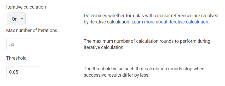
Having iterative calculations enabled may impact the performance of your sheet.
#VALUE!
The #VALUE! error pops up when a function expects a specific type of data (most often numbers) and instead gets something else (most often text):
Function ADD parameter 2 expects number values. But 'two' is a text and cannot be coerced to a number.
As the error message suggests, Google Sheets will do its very best to try to make (coerce) text into a number. That's why this:
Works perfectly. The text " 2 " can be recognised as the number 2.
Some functions (including SUM) ignore data of the wrong type and won't throw the #VALUE! error.
The #VALUE! error comes up a lot when dealing with dates and date-related functions.
In Google Sheets dates are just numbers.
When dates are typed in as text like "thu 16 dec 21" Google Sheets does an amazing job of converting it to a date (12/16/21).
Issues arise when spaces are included "12 /16/21" or there is confusion between formatting dates as mm/dd/yy and dd/mm/yy (you must use the one assigned based on the sheet's locale [ ➜ ➜ ] with the other recognized as text).
How To Fix A #VALUE! Error
Use the error message as a hint before searching through your formula and referenced cells to find where a value you expect to be a number is actually text.
If you can't find the source of a #VALUE! error try looking for blank cells using the ISBLANK, LEN or ISTEXT functions.
Sometimes cells you think are blank are actually full of spaces!
Handling #VALUE! errors using the IFERROR or ERROR.TYPE functions doesn't make sense because you want to know when they happen.
If you do need to know: ERROR.TYPE outputs 3 if its input results in a #REF! error.
'Your Formula Has An Error' Popup
You type in a formula, hit Enter / Return and see this:
There was a problem
It looks like your formula has an error. If you don't want to enter a formula, begin your text with an apostrophe (').
OKNot to worry - this is usually an easy fix.
You'll usually get this error because of a simple typo.
Here's a common one - accidentally including too many parentheses:
They highlight it in red and everything but it's still easy to miss.
Check the last few characters of your formula to make sure there's no unnecessary extras.
Handling Formula Errors
There are a number of functions to help you handle errors in Google Sheets:
IFERROR is the error-based function you'll use the most.
It allows you to predict potential errors and prevent them from affecting other parts of your sheet by providing a backup value if the actual value is an error.
The ERROR.TYPE function is for serious error handling. It returns a number corresponding to the specific error encountered:
- #NULL!
- #DIV/0!
- #VALUE!
- #REF!
- #NAME?
- #NUM!
- #N/A
- All other errors
ERROR.TYPE could be paired with SWITCH or IFS to create a powerful error handling formula that responds differently to each error:
Creates an #N/A error.
It doesn't seem particularly useful but can be used to indicate missing information more effectively than a blank cell and prevent further calculations that depend on it.
Exactly the same as IFERROR but only provides the backup value_if_na if the error is #N/A.
Checks value and returns TRUE if it's an error or FALSE if it's not an error.
Checks value and returns TRUE if it's an #N/A error or FALSE if it's not an #N/A error.
Checks value and returns TRUE if it's any error except #N/A or FALSE if it's an #N/A error or any other value.
FREE RESOURCE
Google Sheets Cheat Sheet
12 exclusive tips to make user-friendly sheets from today:
You'll get updates from me with an easy-to-find "unsubscribe" link.
![MINA Google Sheets Function [With Quiz]](https://kierandixon.com/wp-content/uploads/mina-function-google-sheets.png)
![PROPER Google Sheets Function [With Quiz]](https://kierandixon.com/wp-content/uploads/proper-function-google-sheets.png)
![UPPER Google Sheets Function [With Quiz]](https://kierandixon.com/wp-content/uploads/upper-function-google-sheets.png)